anthe.sevenants

Penalised regression techniques have gained interest in the scientific community for their ability to handle difficult datasets, such as datasets with high-dimensional columns. Unlike in traditional regression, penalised regression introduces a penalty term to the objective function, which attenuates the coefficients of the predictors in the regression. The regression penalty is conducive to conservative coefficient estimates ('shrinkage') and can even cause regression coefficients to come near or even become zero, effectively disabling these predictors and performing variable selection. As such, we can use these techniques to prevent overfitting and create more parsimonious models.

In this article, I will not delve into the background of the different penalised regression techniques and their applications. Rather, I will show how to easily perform lasso, ridge and elastic net regression in the R programming language using ElasticToolsR, a library I wrote to make running such regression analyses much easier. To demonstrate how to use ElasticToolsR, we will model a morphosyntactic alternance in Dutch. We will model whether specific words influence what word order is used in a subclause in Dutch. The required dataset for this tutorial will be provided. While I wrote this library for use in linguistics, there is no reason why it could not be used for other fields.

Disclaimer: this guide was written for ElasticToolsR 1.4. Please refer to the GitHub repository for the latest version and instructions.

In addition, all files for this tutorial are available on GitHub.

ElasticToolsR

What is ElasticToolsR?

My ElasticToolsR library makes it easy to execute lasso, ridge and elastic net regression in R. The main idea is that you have a dataset you would use for 'normal' regression, which you can then convert using my library for use with penalised regression. ElasticToolsR then also allows you to execute these penalised regressions using just a few lines of code.

Installing ElasticToolsR

ElasticToolsR is not available on the CRAN package manager yet. To use it, simply copy the scripts from the GitHub repository to your R project's directory (preferably using git clone). From there, you can simply include the scripts you need. If you do not understand git, you can simply download the latest version of ElasticToolsR as a zip file and copy the scripts to your project's directory from the archive.

Make sure that the ElasticToolsR source files are in your project's directory:

anthe@tutorial:~/Projects/ElasticToolsR-tutorial$ ls -l
-rw-r--r-- 1 anthe anthe 14772 Apr  6 11:49 Dataset.R    <-----
-rw-r--r-- 1 anthe anthe  8403 Apr  6 11:49 ElasticNet.R <-----
-rw-r--r-- 1 anthe anthe   759 Apr  6 11:49 MetaFile.R   <-----

Also, before you start, make sure you have installed all dependencies. In R, run the following command to install glmnet and doMC:

install.packages(c("glmnet", "doMC"))

If you use Windows, doMC might not be available.

Using ElasticToolsR

Imports and dataset

First, we import the required ElasticToolsR scripts. These scripts contain all code I have written and will make your life easier.

source("Dataset.R")
source("ElasticNet.R")

Make sure you copied the right files to your project's directory in the previous steps.

Now, it's time to import our data. Usually, this will be a CSV file of some sorts. We will use a CSV file containing information on 2500 sentences in Dutch. We will use the information in this dataset to model the choice between word orders in Dutch. You can download the CSV file manually here, or run the following command in your R script to download the file automatically:

download.file("https://anthe.sevenants.net/get/elastic-tools-r-tutorial/dataset.csv", "dataset.csv")

You can see that the CSV file is now in our project's directory:

anthe@tutorial:~/Projects/ElasticToolsR-tutorial$ ls -l
-rw-r--r-- 1 anthe anthe 14772 Apr  6 11:49 Dataset.R
-rw-r--r-- 1 anthe anthe  8403 Apr  6 11:49 ElasticNet.R
-rw-r--r-- 1 anthe anthe   759 Apr  6 11:49 MetaFile.R
-rw-r--r-- 1 anthe anthe   205 Jul  3 14:12 Tutorial.R
-rw-r--r-- 1 anthe anthe 91212 Jul  3 11:28 dataset.csv <-----

We now load our dataset into the object df using read.csv:

df <- read.csv("dataset.csv")

When we look at the dataset, we see that we have four columns:

str(df)

'data.frame':   2500 obs. of  4 variables:
 $ participle: chr  "gedaan" "rechtgezet" "gestart" "gebleven" ...
 $ order     : chr  "green" "red" "red" "green" ...
 $ country   : chr  "BE" "BE" "NL" "NL" ...
 $ edited    : logi  FALSE TRUE TRUE TRUE TRUE TRUE ...

• participle: the verb in our Dutch sentence
• order: the word order of the sentence
• country: the country the sentence is from (BE/NL - Belgium/The Netherlands)
• edited: whether the sentence comes from an edited text genre

order is the word order we want to model. We want to know what influences the choice between both possible orders (here, there is a choice between a 'red' and 'green' order). participle contains the different verbs from our Dutch sentences. Since there are many different possible words, we have to use penalised regression, since regular regression techniques cannot fit models for so many data levels. country has only two possible values, just like edited.

ElasticToolsR expects the response variable column (order for us) to be a factor. Therefore, we explicitly define it as a factor:

df$order <- as.factor(df$order)

In addition, any 'high-dimensional' column should also be defined as a factor. Our participle column is an example of such a column, since it contains many possible levels for many different verbs:

df$participle <- as.factor(df$participle)

We include two other predictors in our analysis as well. Both country and edited have a possible influence on the choice between either word order, and we want to make sure that we correct for this: we need these sources of variation to also be accounted for. In ElasticToolsR, such other predictors can be either factors, logical values or continuous numeric data types.

country has only two values, so it is not high dimensional. Its values are not strictly logical (there is no TRUE/FALSE distinction), so we define this column as a factor:

df$country <- as.factor(df$country)

edited has only two values, so it is not high dimensional. Its values are strictly logical (there is a TRUE/FALSE distinction), so we define this column as a logical data type:

df$edited <- as.logical(df$edited)

Now, we can build an ElasticTools dataset. In contrast to regular regression techniques, a tabular dataset cannot be used 'as-is' for analysis with penalised regression. Instead, the dataset has to be supplied in a matrix form. This is why we define an ElasticTools dataset, because the library will take care of the matrix conversion under the hood automatically.

ds <- dataset(df=df,
              response_variable_column="order",
              to_binary_columns=c("participle"),
              other_columns=c("country", "edited"))

We define order as our response variable and make clear that participle is a high-dimensional column that needs to be converted to binary predictors (see below). For our other columns, we supply a character vector with country and edited.

To understand what ElasticTools does under the hood, consider the following snippet from our dataset:

order	participle	country	edited
green	gedaan	BE	FALSE
red	rechtgezet	BE	TRUE
red	gestart	NL	TRUE

In the matrix form, each high-dimensional column is converted so that each unique value of that column becomes its own predictor. In our case, all unique values of the column participle will become binary predictors, each predictor indicating whether that participle occurs in the cluster or not. This means our matrix will be inherently sparse, since each cluster can only feature one participle. Binary predictors such as country are also converted to a binary column in the matrix, and simply indicate a deviation from the reference level. For example, if Belgium is the reference level, a Belgian attestation will be encoded as 1, and a Netherlandic attestation as 0. The edited column is taken over as-is as a binary column. The response variable order is also encoded as a binary variable, as is typical in logistic regression, but it is not a part of the input matrix. The input matrix for our dataset snippet would look as follows:

is_gedaan	is_rechtgezet	is_gestart	is_BE	is_Edited
1	0	0	1	0
0	1	0	0	1
0	0	1	1	1

The response variables would be encoded as [ 0, 1, 1 ] with the red order as the reference level.

Running the penalised regression

Before we can run penalised regressions, we define an elastic_net object. This object creates the matrix form I discussed earlier under the hood. It also saves the response variables so they are ready for use. This is done in advance because it can take some time depending on the size of your dataset.

net <- elastic_net(ds=ds,
                   nfolds=10,
                   type.measure="deviance")

• ds: the ElasticTools dataset to use for the regressions
• nfolds: the number of folds used in cross-validation (see below)
• type.measure: the loss used for cross-validation (this is a setting for nerds)

The nfolds parameter is important for cross-validation. This process is necessary, since both lasso and ridge regression use the lambda parameter to determine the severity of the penalty applied during the model fitting process. This lambda value can range from 0 (no penalty) to +\infty (maximal penalty). The question then arises how one decides what value to use for lambda in order to obtain the best possible model. To compute lambda, we typically rely on k-fold cross-validation, a common practice in the machine learning field. We divide our dataset into k 'folds', effectively 'slices' of data. For example, in 10-fold cross validation, the dataset will be divided into ten parts. First, we use the nine folds to fit the model ('training set') and try a wide array of different lambda values. To examine how well each lambda value performs, we predict values using the fitted model and test how much the predictions deviate from the real values in the remaining fold ('testing set'). We then repeat this process nine more times, each time with a different fold used as a testing set. This enables us to get a global estimation of how well each possible lambda value performs, which helps combat overfitting. The lambda value which produces the best predictions across all fold combinations is chosen to fit a model on the entire dataset.

Now, we can choose what type of penalised regression we want to run. I will show all types.

1. To run a ridge regression, use the $do_ridge_regression() method. This will return a regression fit.

    fit <- net$do_ridge_regression()

2. To run a lasso regression, use the $do_lasso_regression() method. This will return a regression fit.

    fit <- net$do_lasso_regression()

3. To run a lasso regression, use the $do_lasso_regression() method. This will return a regression fit. Elastic net regression leverages the strengths of ridge and lasso. With an additional parameter alpha (\alpha), we regulate the split between lasso and ridge (alpha encodes how much lasso is used).

    fit <- net$do_elastic_net_regression(alpha=0.5)

   You can let ElasticToolsR come up with the ideal alpha value automatically. The 'ideal' alpha value is defined here as the value which yields the model which produces the best predictions. To automatically find the best alpha value, use the $do_elastic_net_regression_auto_alpha method.

    collection <- net$do_elastic_net_regression_auto_alpha(k=10)

   k encodes how many alpha values we try. With k = 10, we create models in increments of 0.1 from 0 to 1.

   The method will return a list with two named elements:

   • $results: a data frame containing the results of the cross validation
   • $fits: a list of regression fit objects associated with the different parameter values tried

   If we ask for the results table, we can see for each model the library tried how big its 'loss' is. This loss represents numerically how far our predictions are from the truth:

    collection$results

       X_id alpha     loss   intercept  dev.ratio nzero     lambda
    1     1   0.0 1.253967  0.34700411 0.15627736   807 0.64198697
    2     2   0.1 1.228682  0.03085716 0.10539140   263 0.11482897
    3     3   0.2 1.228036 -0.05518595 0.08844725   119 0.06915595
    4     4   0.3 1.228302 -0.09332068 0.08022520    64 0.05059905
    5     5   0.4 1.226397 -0.13059705 0.08268216    62 0.03794928
    6     6   0.5 1.228948 -0.13290064 0.07498525    55 0.03331943
    7     7   0.6 1.228117 -0.15114022 0.07598217    55 0.02776620
    8     8   0.7 1.227532 -0.16482054 0.07670159    55 0.02379960
    9     9   0.8 1.227099 -0.17546461 0.07724461    55 0.02082465
    10   10   0.9 1.226765 -0.18398398 0.07766869    55 0.01851080
    11   11   1.0 1.226501 -0.19094954 0.07801113    54 0.01665972

   We also see some other properties about the models (intercept, deviance ratio, number of zero coefficients, ideal lambda). We select the model fit with the lowest loss:

    lowest_loss_row <- collection$results[which.min(collection$results$loss),]
    fit <- collection$fits[[lowest_loss_row[["X_id"]]]]

   We see that this corresponds to the model with 0.4 as its alpha value:

    lowest_loss_row$alpha

    [1] 0.4

Regardless of what penalised regression technique you used, you should now have a fit object containing the penalised model of the word orders in Dutch:

fit

Call:  cv.glmnet(x = x, y = y, type.measure = type.measure, foldid = ds$df$foldid, parallel = parallel, alpha = alpha, family = "binomial") 

Measure: Binomial Deviance 

     Lambda Index Measure      SE Nonzero
min 0.02383    26   1.215 0.01475     313
1se 0.03795    21   1.226 0.01243      62

This fit object is a glmnet fit S3 object which contains all kinds of information on your penalised model. You can consult the glmnet manual in order to find out more about what information can be retrieved from this object, but for the sake of thoroughness, I will give an overview of the most important attributes.

1. fit$lambda contains all lambda values the glmnet library has tried.

    fit$lambda

    [1] 2.439408e-01 2.222698e-01 2.025239e-01 1.845323e-01 1.681389e-01 1.532019e-01 1.395919e-01 1.271909e-01 1.158916e-01
    [10] 1.055961e-01 9.621527e-02 8.766777e-02 7.987961e-02 7.278332e-02 6.631745e-02 6.042599e-02 5.505791e-02 5.016672e-02
    [19] 4.571005e-02 4.164929e-02 3.794928e-02 3.457798e-02 3.150616e-02 2.870724e-02 2.615697e-02 2.383326e-02 2.171598e-02
    [28] 1.978679e-02 1.802898e-02 1.642734e-02 1.496798e-02 1.363827e-02 1.242668e-02 1.132273e-02 1.031685e-02 9.400328e-03
    [37] 8.565228e-03 7.804317e-03 7.111003e-03 6.479281e-03 5.903680e-03 5.379213e-03 4.901339e-03 4.465917e-03 4.069177e-03.
    ...

2. fit$lambda.1se and fit$lambda.min: the fit object gives us two lambda values, one '1se' and one 'min'. lambda.min is the value of lambda that gives the minimum mean cross-validated error. lambda.1se is the value of lambda that gives the most regularised model such that cross-validated error is within one standard error of the minimum. While you would think that we would use lambda.min because it yields the best results, we typically choose lambda.1se:

   We often use the “one-standard-error” rule when selecting the best model; this acknowledges the fact that the risk curves are estimated with error, so errs on the side of parsimony.

   Friedman, Hastie, and Tibshirani (2010)

   Basically, we choose lambda.1se to avoid overfitting. This yields the 'somewhat' best model.

    fit$lambda.1se

    [1] 0.03794928

3. fit$cvm contains the losses for all lambda values the glmnet library has tried. The order in fit$lambda is the same in all other vectors, so fit$cvm[3], for example, corresponds to the model with a lambda of fit$lambda[3].

    fit$cvm

    [1] 1.305015 1.301967 1.297840 1.294060 1.290600 1.287267 1.283348 1.278998 1.274980 1.270867 1.266883 1.263127 1.259630
    [14] 1.256091 1.252531 1.248577 1.243916 1.238915 1.234411 1.230207 1.226397 1.223079 1.220430 1.217654 1.215385 1.214642
    [27] 1.215700 1.217727 1.220006 1.223147 1.227338 1.232492 1.238610 1.245413 1.252748 1.260708 1.269306 1.278519 1.287931

4. fit$nzero contains the number of zero coefficients for all lambda values the glmnet library has tried.

    fit$nzero

    s0  s1  s2  s3  s4  s5  s6  s7  s8  s9 s10 s11 s12 s13 s14 s15 s16 s17 s18 s19 s20 s21 s22 s23 s24 s25 s26 s27 s28 s29 s30 
     0   1   1   1   1   1   2   2   2   3   3   4   4   6   9  15  17  25  33  55  62 117 149 262 306 313 342 375 528 554 572 
    s31 s32 s33 s34 s35 s36 s37 s38 s39 s40 s41 s42 s43 s44 s45 s46 s47 s48 s49 s50 s51 s52 s53 s54 s55 s56 s57 s58 s59 s60 s61 
    578 597 600 606 607 639 771 771 771 775 778 779 781 782 783 789 789 795 795 795 799 799 799 802 802 802 802 802 802 802 802 

5. fit$glmnet.fit$a0 contains the intercepts for all lambda values the glmnet library has tried.

    fit$glmnet.fit$a0

    s0          s1          s2          s3          s4          s5          s6          s7          s8          s9 
    0.58231538  0.56260521  0.54349648  0.52503647  0.50726396  0.49020937  0.43213294  0.37450158  0.31970146  0.26847456 
    s10         s11         s12         s13         s14         s15         s16         s17         s18         s19 
    0.22013423  0.17442349  0.13123442  0.08973719  0.05074503  0.01499882 -0.01720815 -0.04919622 -0.07956811 -0.10734734 

6. fit$glmnet.fit$dev.ratio contains the deviance ratios for all lambda values the glmnet library has tried.

    fit$glmnet.fit$dev.ratio

    [1] -2.416147e-14  3.470630e-03  6.669484e-03  9.601657e-03  1.227506e-02  1.469993e-02  1.843219e-02  2.185953e-02
    [9]  2.491872e-02  2.841497e-02  3.166966e-02  3.459647e-02  3.774993e-02  4.082313e-02  4.418658e-02  4.864913e-02
    [17]  5.381319e-02  5.935548e-02  6.600811e-02  7.351583e-02  8.268216e-02  9.766247e-02  1.129444e-01  1.324309e-01

7. fit$index shows you the indices of lambda.min and lambda.1se. You can use them to index the vectors above and find associated values for models with these lambda values.

    fit$index

    Lambda
    min     26
    1se     21

You can use these attributes of the regression fit to report on your model in scientific papers. Especially the lambda value, number of zero coefficients and intercept are important.

Retrieving coefficients and their values

The most important aspect of a regression analysis is the coefficients it produces, since they tell us about how or whether the model corrects for the presence of specific variables. You can get the names of the coefficients and their associated values with the following code:

coefficients_with_labels <- net$attach_coefficients(fit)

This returns a data frame which contains all the coefficients of the fitted model and their associated features:

head(coefficients_with_labels)

    coefficient  feature
141  -1.5774912 verboden
78   -1.4346466 getrouwd
308  -1.0274115   gewend
465  -0.9937847 geregend
205  -0.9846635  omringd
256  -0.9496847  gestopt

Analysing coefficients using Rekker

Because it is really cumbersome to inspect these coefficients manually, I built visual frontend called Rekker, which allows you to visualise regression coefficients. We can use this tool as a basis for our analysis.

To load our coefficients into Rekker, we first have to export the coefficients and their labels to a CSV file:

write.csv(coefficients_with_labels, "coefficients.csv", row.names=FALSE)

This produces a new file called 'dataset.csv' in our project's directory:

anthe@plain:~/Projects/ElasticToolsR-tutorial$ ls -l
-rw-r--r-- 1 anthe anthe 14772 Apr  6 11:49 Dataset.R
-rw-r--r-- 1 anthe anthe  8403 Apr  6 11:49 ElasticNet.R
-rw-r--r-- 1 anthe anthe   759 Apr  6 11:49 MetaFile.R
-rw-r--r-- 1 anthe anthe  1381 Jul  3 16:32 Tutorial.R"
-rw-r--r-- 1 anthe anthe 12347 Jul  3 16:39 coefficients.csv <-----
-rw-r--r-- 1 anthe anthe 69869 Jul  3 14:17 dataset.csv

Now, we can open Rekker. We load our coefficients.csv file into Rekker:

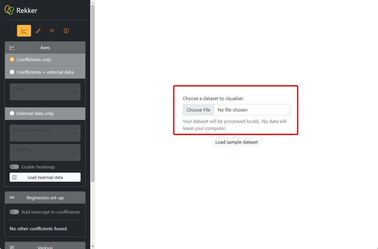
The coefficients are now rendered visually on a dot plot. We can see for each verb individually whether there is a pull towards either word order. Since the red order is the reference level (= 1), the negative coefficients represent pulls towards the green word order.

In the left sidebar, we can see the influence of our other predictors (order and country). These values can also be toggled to be added to the coefficient values.

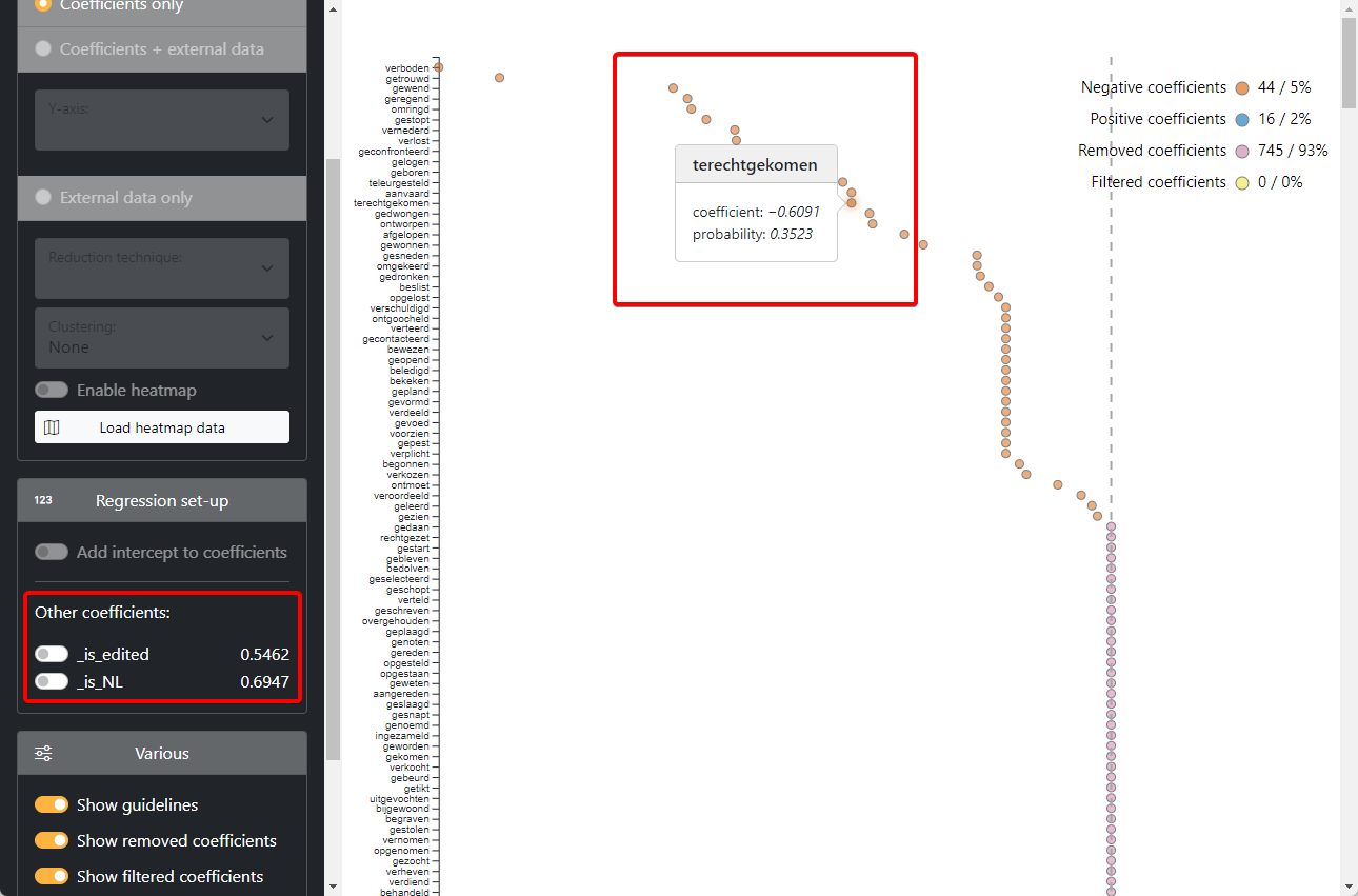
We can now investigate the correction the model applies for each verb within the Rekker program.