For NLP applications or linguistic research, it is useful to represent words as continuous vectors. Continuous vector representations allow for (pseudo) semantic generalisation across vectors, and are favoured over naive one-hot encoding. Still, it can be quite confusing to work with these vectors, as they are high-dimensional and cannot be inspected 'as-is'. Instead, the numeric information is usually condensed into a two-dimensional plot which attempts to capture semantic distance information from the vectors as well as possible. Through these two-dimesional plots, one can then attempt to glean semantic patterns and make linguistic inferences. In this article, I will explain how to use my DistributionalSemanticsR library in order to...
- ...extract semantic vectors from snaut, a prebuilt source of semantic vectors for English and Dutch;
- ...reduce those vectors to two dimensions, so they can be visualised on a 2D plot.
1. Installation
DistributionalSemanticsR is not available on the CRAN package manager (yet). To use it, first download the DistributionalSemanticsR repository ZIP file. Then, copy all .R files to your own project's directory. It should look like this:
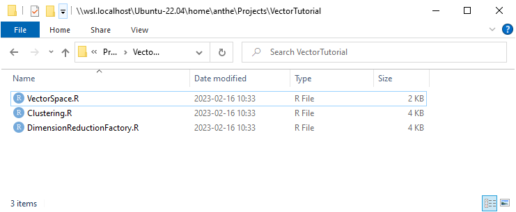
Now, we can create our own R script in the same directory and write our own code.
2. Importing DistributionalSemanticsR in your own script
Before we can start using DistributionalSemanticsR, we first have to install its dependencies. To do so, run the following command:
install.packages("vegan", "Rtsne", "umap")Then, we can import the library's files. Fortunately, this is really simple:
source("VectorSpace.R")
source("DimensionReductionFactory.R")
We only use VectorSpace.R and DimensionReductionFactory.R. Clustering.R is only used for clustering, which we will not do here.
3. Downloading the snaut semantic vectors
While you can build your own semantic vectors (or use an AI to build them for you), we will keep things simple by just downloading a prebuilt matrix with vectors for almost any English word you can think of. I have pre-selected this archive. Beware, semantic vectors are large, and the linked archive contains at least 150.000 of them. This means the archive's file size is large and you will have to wait for it to download.
Once the download is finished, place the .gz archive in your project's directory. You do not have to extract it.
4. Defining a vector space in R
We can now turn back to R to define a vector space using the semantic vectors we just downloaded. To do this, we first load the matrix from the archive:
vector_matrix <- as.matrix(
                  read.table(
                   gzfile('english-all.words-cbow-window.6-dimensions.300-ukwac_subtitle_en.w2v.gz'),
                  sep=' ',
                  row.names=1,
                  skip = 3))
We tell R to open the .gz archive using gzfile. Then, we read its contents as a table (read.table), with a space (' ') as the separator between the values. We use the first line as the row names and skip the first three rows (they contain junk data - do not worry about this). Then, we convert this table into a matrix (as.matrix). Since the matrix is very large, the loading process can take quite a long time.
After our vector matrix has been loaded, we can turn it into a vector space:
my_vector_space <- vector_space(space=vector_matrix)5. Getting the distributional vectors for a list of words
Now that our vector space is defined, we can use it to fetch the vectors for the specific words we are interested in. First, we create a vector of all the words we want to retrieve semantic vectors of:
my_words <- c("cake", "biscuit", "crisps", "pizza", "broccoli", "carrot", "beef",
              "cola", "lemonade", "toast", "computer", "printer", "keyboard")
Then, we tell R we want to use the vector space we defined in step 4 to retrieve our distributional vectors:
distributional_coords <- my_vector_space$get_distributional_values(my_words)If we inspect the distributional_coords object, we see that, indeed, we have a matrix of 13 high-dimensional vectors:
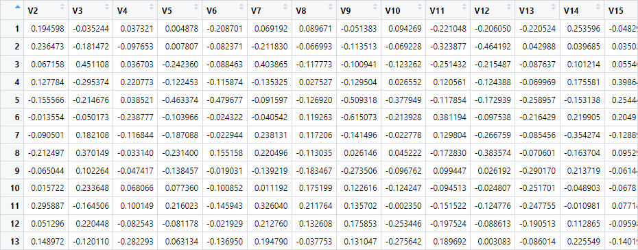
The first vector row corresponds to cake, the second to biscuit, and so on.
6. Reducing the semantic space to two dimensions for plotting purposes
With your distributional coordinates collected, you can now define a DimensionReductionFactory instance. In this metaphorical 'factory', your dimension-reduced coordinates will be produced. To define a factory, you just give it your distributional coordinates:
dim_reduce <- dimension_reduction_factory(distributional_coords)In the background, the program will now create a so-called distance matrix. This matrix contains the pairwise distances between all our semantic vectors. In practice, this means that the distance between cake and biscuit will be computed, but also the distance between cake and crisps, pizza, broccoli, carrot .. etc. In this way, every combination gets a measure of 'how far' the semantics of the elements in the combination lie. Of course, this all happens under the hood if you use DistributionalSemanticsR, but for clarity's sake, I have brought up the hidden distance matrix here:
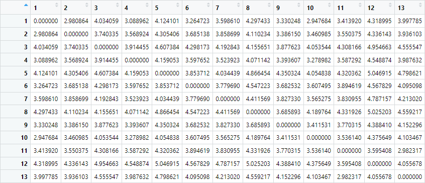
You can see that our distance matrix contains 13 rows and 13 columns, since it holds the distances between our 13 words. Here as well, the first row/column corresponds to cake, the second to biscuit, and so on. On the diagonal, words are compared to themselves, so of course the distance here is always 0. It is on the distance matrix , like the one shown above, that dimension reduction is applied. Full vectors are not used.
With this bit of theoretical background out of the way, we can now tell R to run dimension reduction on our distance matrix using any of the three supported dimension reduction techniques in DistributionalSemanticsR (MDS, TSNE and UMAP). I will demonstrate MDS in this case:
coords.mds <- dim_reduce$do_mds()For TSNE or UMAP, replace do_mds with do_tsne or do_umap respectively - it is possible that you get data-related errors with other techniques, since our distance matrix only contains 13 words.
Still, yes, it is that simple. If we inspect our coords.mds object, we indeed see our two-dimensional coordinates:
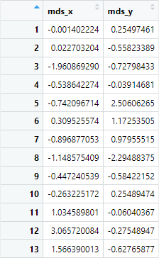
Now, we can add our labels back onto the coordinates...
coords.mds$word <- my_words...and we can finally visualise our words on a plot:
plot(coords.mds$mds_x, coords.mds$mds_y, ylim=c(-2.5, 2.5))
text(coords.mds$mds_x, coords.mds$mds_y, labels=coords.mds$word, pos=1)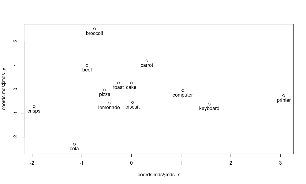
As you can see, the food-related words are shown on the left side of the plot. Computer-related words are on the right side of the plot. This shows that in some way, this semantic distinction is captured in the snaut distributional vectors. It is more difficult to find fine-grained distinctions between the food-related words, but of course this plot is only based on a distance matrix of 13 words. Try experimenting with more words and larger plots, as well as other dimension reduction techniques. What results do you get?